Densecrf与图像分割
在图像分割中,在FCN之前,流行的是以概率图模型为代表的传统方法. FCN出来之后一段时间,仍然流行的是以FCN为前端,CRF为后端优化. 随着网络的发展,CRF的优化已慢慢不再具有明显的性能提升. 不谈理论细节,仅示例介绍与使用.
Dense-crf 图示
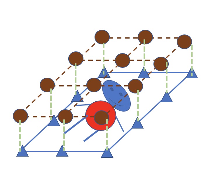
如上图所示,有一张有一个小人的图像,需要对图像中的各个像素进行分类,△ 代表一个像素,像素集合为$X$,每一个像素所对应隐式类别 ⭕️ 为 $z$, 组成类别集合 $Z$. 观测即为像素的颜色、位置特征,需要推论的隐变量即为每个像素的类别.
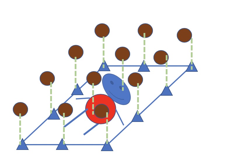
假如每一个像素的类别只和自己的像素特征相关. 如下图所示. 意味着对每一个像素单独进行一次分类,直观的讲,仅从一个像素所具有的特征是无法有效的对像素进行分类的. 自然而然的可以想到,一个像素的类别应该与它的邻域甚至所有像素相关.
下图所示,一个像素的类别信息由所有像素共同决定. 这实际上就是FCN所完成的工作.
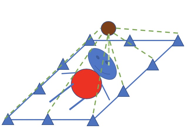
FCN只能解决图像像素和类别之间的相关关系,也就是$X$ 和 $Z$ 的联合建模. 而实际上每个像素的类别之间也存在关联关系,即图像平滑性–每一个像素的类别可能和临近点的类别很类似.这是FCN所欠缺的,也正是Dense-crf所弥补的. ref[1]
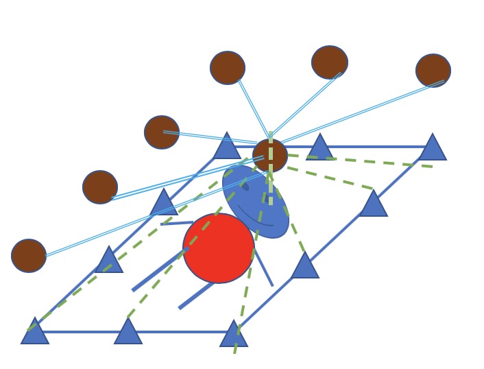
因此,在上图的基础上,一个像素的类别不光受与所有像素相关. 同时与所有像素的类别相关. 故称为dense-crf. 如下图所示(由于链接太多,仅画出示意. 任意一对像素的类别信息都互联,任意单个像素的类别与所有像素相连)
Dense-crf 公式
$$E(z)=\sum_i \psi_u(X, z_i) + \sum _{i<j} \psi_p(X,z_i,z_j)$$
其中,第一项为与像素自身类别相关的 unary 能量函数. 后一项为 pairwise 函数中每一个像素的类别信息都与其它像素的类别信息、所有像素的信息相关. pairwise 函数展开为
$$\psi_p(z_i, z_j) = \mu(z_i,z_j)\sum ^k _{m=1} w ^{(m)} k ^{(m)} (x_i,x_j)$$
$\mu(z_i,z_j)$ 为标签一致性因子. 其中:
$$k ^{(m)}(f_i,f_j)=w ^{(1)} exp(-\frac{|p_i - p_j| ^2}{2\theta ^2 _\alpha} - \frac{|I_i - I_j| ^2}{2\theta ^2 _\beta}) + w ^{(2)} exp(-\frac{|p_i - p_j| ^2}{2\theta ^2 _\gamma})$$
上式中,第一项为appearance kernel, 第二项为smooth kernel. appearance核中第一项 $p$ 代表像素的位置, 第二项 $I$ 为像素强度值.
pydensecrf 使用demo
此处使用开源实现的pydensecrf. 安装及代码
demo1: DenseCRF2D + 二分类
def dense_crf(img, probs, n_labels=2):
    h = probs.shape[0]
    w = probs.shape[1]

    probs = np.expand_dims(probs, 0)
    # 概率作为unary, 通道数和类别数相同
    probs = np.append(1 - probs, probs, axis=0)

    d = dcrf.DenseCRF2D(w, h, n_labels)
    # unary 为负对数概率
    U = -np.log(probs)
    U = U.reshape((n_labels, -1))
    U = np.ascontiguousarray(U)
    img = np.ascontiguousarray(img)

    U = U.astype(np.float32)
    d.setUnaryEnergy(U)

    d.addPairwiseGaussian(sxy=20, compat=3)  #
    d.addPairwiseBilateral(sxy=30, srgb=20, rgbim=img, compat=10)

    Q = d.inference(5)
    # 获得map对应的标签
    Q = np.argmax(np.array(Q), axis=0).reshape((h, w))

    return Q

probs = infer_model.predict(image, batch_size=1)
probs = np.squeeze(probs, axis=0)
probs = sigmoid(probs)
mask = dense_crf(np.array(image_ori).astype(np.uint8), probs)
此实例为前景背景分割二分类,网络输出经过 $sigmoid$ 激活函数的单通道概率.
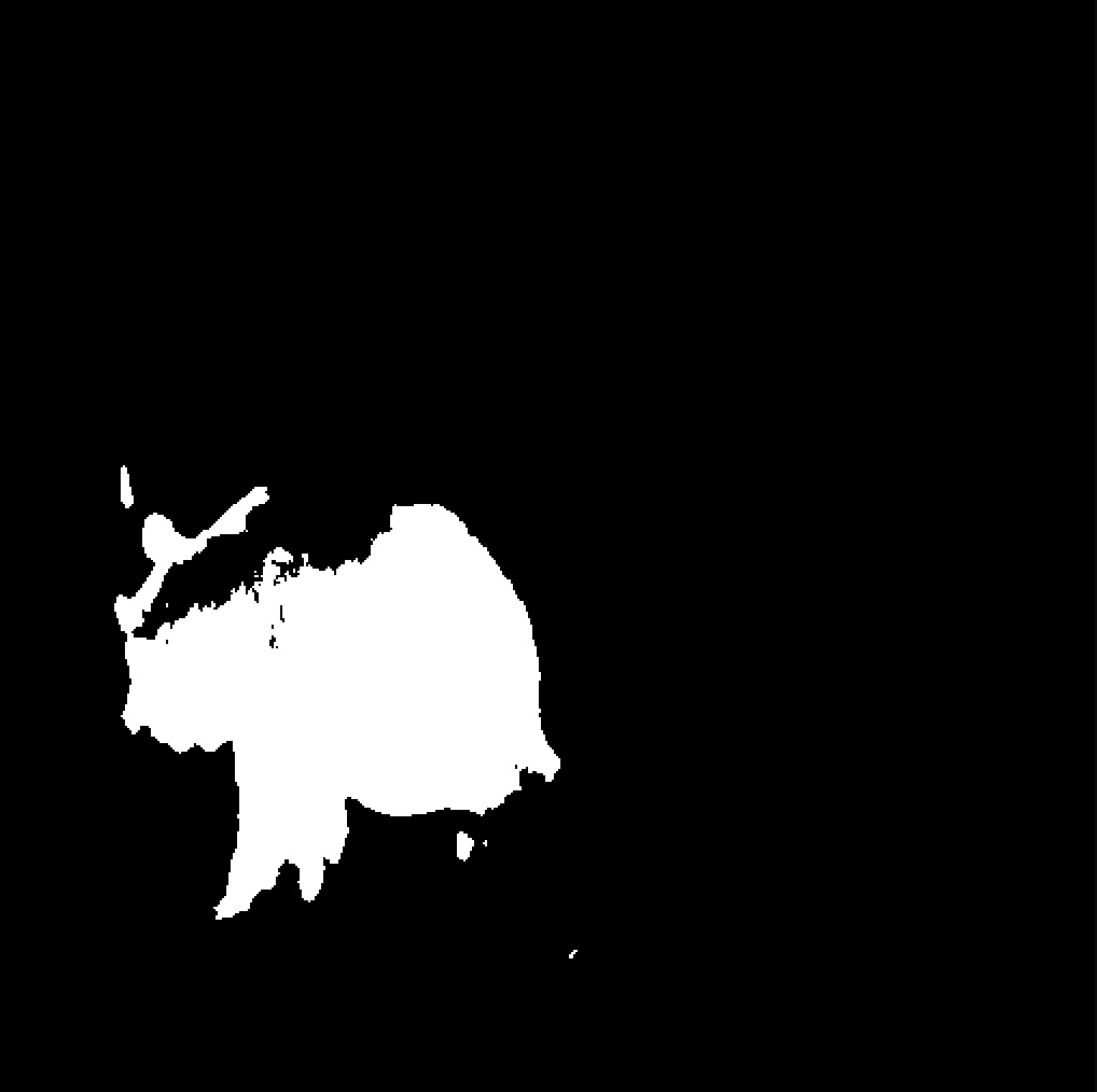
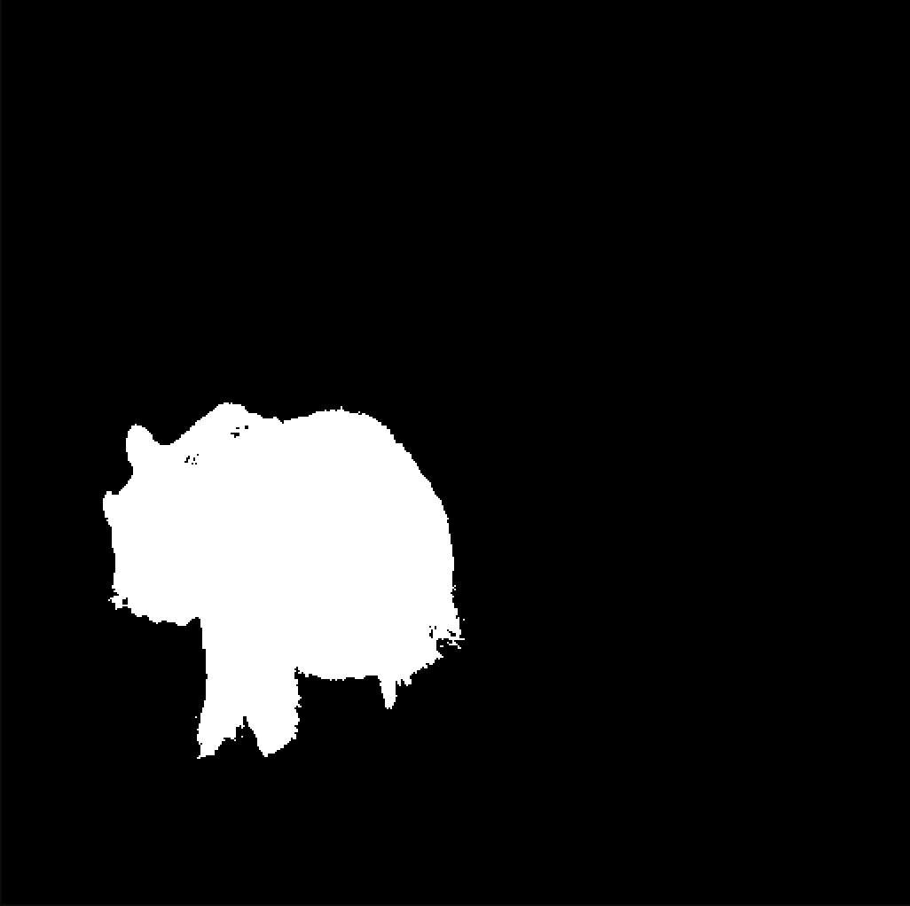
左图为网络直接分割后得到的结果,右图为densecrf处理后的结果.
demo2: DenseCRF + 多分类
pascal voc 21类语义分割测试,使用deeplab-resnet
def dense_crf(probs, img, n_labels=21):
    # unary shape 为(n_labels, height, width)
    probs = probs.transpose((2, 0, 1))
    unary = softmax_to_unary(probs)
    unary = np.ascontiguousarray(unary)
    d = dcrf.DenseCRF(img.shape[0] * img.shape[1], n_labels) # width, height, n_labels
    d.setUnaryEnergy(unary)

    # This potential penalizes small pieces of segmentation that are
    # spatially isolated -- enforces more spatially consistent segmentations
    feats = create_pairwise_gaussian(sdims=(10, 10), shape=img.shape[:2])
    d.addPairwiseEnergy(feats, compat=3,
                        kernel=dcrf.DIAG_KERNEL,
                        normalization=dcrf.NORMALIZE_SYMMETRIC)

    # This creates the color-dependent features --
    # because the segmentation that we get from CNN are too coarse
    # and we can use local color features to refine them
    feats = create_pairwise_bilateral(sdims=(50, 50), schan=(20, 20, 20),
                                      img=img, chdim=2)

    d.addPairwiseEnergy(feats, compat=10,
                        kernel=dcrf.DIAG_KERNEL,
                        normalization=dcrf.NORMALIZE_SYMMETRIC)
    Q = d.inference(5)
    Q = np.argmax(Q, axis=0).reshape((img.shape[0], img.shape[1]))
    return Q


res = dense_crf(probs, img)
res = res[np.newaxis,:,:,np.newaxis]
msk = decode_labels(res, num_classes=21) #code from deeplab-resnet
im = Image.fromarray(msk[0])
im.show()

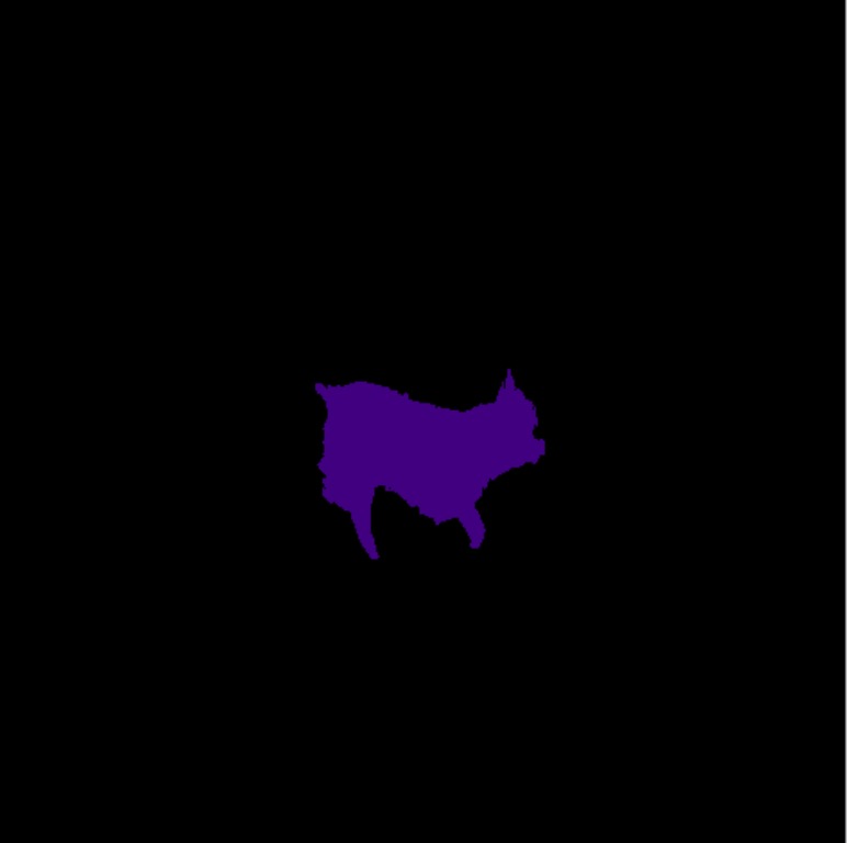
左图为网络分割结果,右图为dense-crf优化结果,可以看出效果甚至变差了. 网络够强的情况下,添加crf优化没有太大必要.
参数说明
网络的概率输出作为 $unary$ 项.
- addPairwiseGaussian. 仅使用位置特征
- addPairwiseBilateral. 使用颜色与位置特征
$sxy (sdims), srgb (schan)$ 分别对应 $pairwise$ 函数中的 $\theta _\beta , \theta _\alpha$ , 可逐通道指定. 对 $chdim$ ,$rgb$ 图像设为2, 单通道图像设为 -1.
参考文献
- 深度学习轻松学:核心算法与视觉实践
- 🍉📚. 周志华
- pydensecrf