SSD发表在2016ECCV, 是one-stage目标检测算法中经典的框架之一. 其精度优于yolo-v1, 在yolo-v2之后被超越.

SSD 具有以下特点:

• 从YOLO中继承了将detection转化为regression的思路，一次完成目标定位与分类
• 基于Faster RCNN中的Anchor，提出了相似的Prior box
• 加入基于特征金字塔（Pyramidal Feature Hierarchy）的检测方式，即在不同感受野的feature map上预测目标

1. MultiBox Detector

SSD 的 multibox 就是每个检测子预测多个shape的先验框(即faster-rcnn 中的anchor-box).

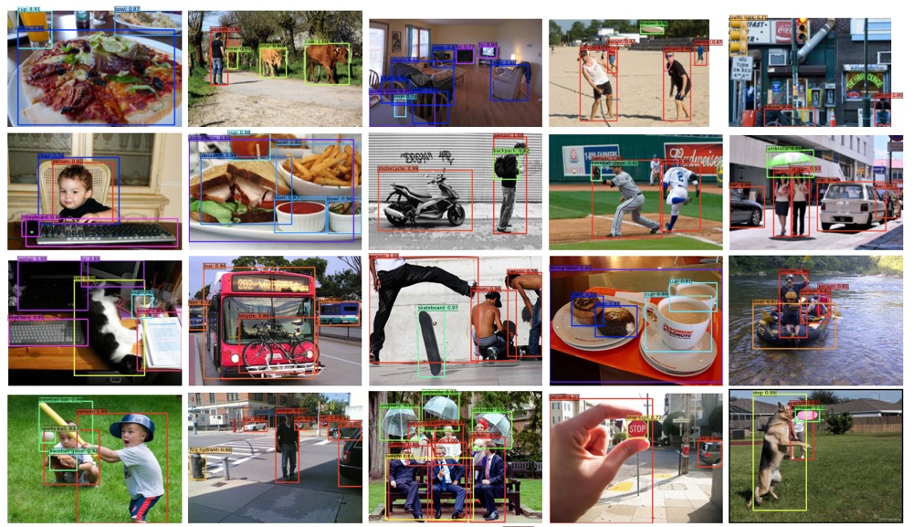
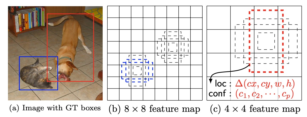
• 如上图, 为某些不同尺度下得到的 feature map(每一个像素点为一个location). SSD 会在多个尺度下运用 multibox 检测, 多个尺度下输出检测结果, 可以针对于不同大小的物体, 提高召回.
• 每一个 location 都会得到 k 个 bounding-box, 每个bounding-box 具有不同的尺寸与纵横比(anchor-box). SSD 中, 不同尺度下分配的 bounding-box 个数不同.
• 每个bounding-box 均预测 C 个类别的概率以及相对于 default box 中心 $cx, cy$ 和 宽高 $w, h$ 的偏移量.

2. SSD Network Architecture

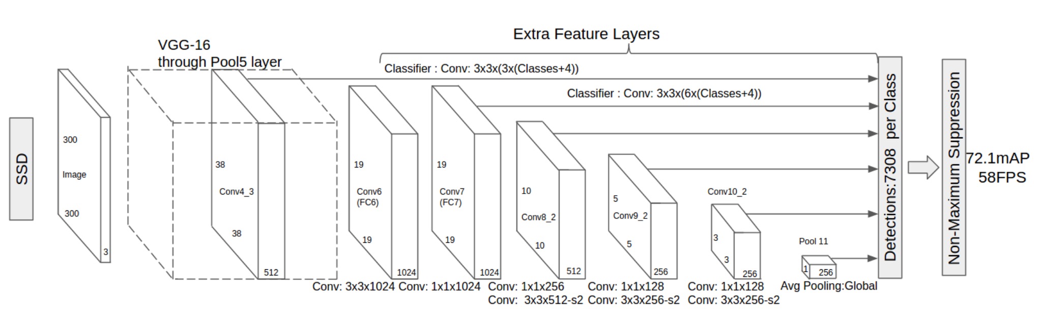
SSD 300(输入尺寸为300 * 300) 网络结构图如上, 其基网络为 VGG16, Fc6 与 Fc7 两个全连接层改为卷积层. SSD 一共在6 个尺度下进行了检测, 共得到7308个 bounding-box, 可以看出远超 yolo-v1 的98个box.

• 在 conv4_3 , feature map 为 38 * 38. 在此层分配了4个default box, 共可检测 38 * 38 * 3 = 4332 个 bounding box.
• conv_7 层, 每个location分配6个default box, 共可检测 19 * 19 * 6 = 2166 个 bounding box. 以下每层均为每个location分配6个default box.
• conv8_2 层, 可检测 10 * 10 * 6 = 600 个bounding box.
• conv9_2 层, 可检测 5 * 5 * 6 = 150 个bounding box.
• conv10_2 层, 可检测 3 * 3 * 6 = 54 个bounding box.
• 最后一层, 可检测 1 * 1 * 6 = 6 个bounding box.

SSD 一共可检测 4332 + 2166 + 600 + 150 + 54 + 6 = 7308. 感受野小的浅层检测小目标.

3. Loss

$$L(x,c,l,g) = \frac{1}{N}(L _{conf} (x,c) + \alpha L _{loc} (x,l,g))$$

损失函数包含两项, 分类损失与坐标损失. $N$ 为匹配的default box.

Location loss 为 smooth l1 损失, 其中 $l$ 为预测框, $g$ 为 gt, 类似于faster rcnn 计算偏移值:

$$L _{loc} (x,l,g) = \sum ^ N _{i\in Pos} \sum _ {m \in {cx,cy,w,h}} x ^k _{ij} smooth _{L1} (l ^m _i - \bar g ^m _j)$$

$$\bar g _j ^{cx} = (g _j ^{cx} -d _i ^{cx})/d _i ^w , g _j ^{cy} = (g _j ^{cy} -d _i ^{cy})/d _i ^h$$

$$ \bar g ^w _j = log \frac{g ^w _j}{d ^w _i} , \bar g ^h _j = log \frac{g ^h _j}{d ^h _i}$$

confidence loss 如下, 为多类softmax loss:

$$L _{conf} (x,c) = - \sum ^ N _{i \in {Pos}} x ^p _{ij} log(\bar c ^p _i) - \sum _{i \in {Neg}} log(\bar c ^0 _i), \bar c ^p _i = \frac{exp(c ^p _i)}{\sum _p exp(c ^p _i)}$$

$$x ^p _{ij} = {1, 0}$$

代表第 $i$ 个 default box 匹配到第 $j$ 个类别为$p$的GT box.

4. scales and aspect ratios for default boxes

$$s_k = s _{min} + \frac{s _{max} -s _{min}}{m-1}(k-1), k \in[1,m]$$

$m$ 为预测时使用的特征图的数量, 本文中使用了6个尺度下的特征图($m=6$). 文字设定 $s _{min}=0.2, s _{max} =0.95$ , 意味着最低层的 scale 为0.2, 最顶层scale 为0.95. 中间层规则分开.

对于每一个scale, 有5个非正方形的长宽比:

$$ a _r \in {1,2,3,\frac{1}{2},\frac{1}{3}}, (w ^a _k=s_k \sqrt a_r), (h ^a _k= s_k / \sqrt a_r)$$

对于长宽比为1, 增加一个default box, 其 scale 为 $s^* _k = \sqrt {s_ks_k + 1}$.

5. Matching strategy：

• 首先，寻找与每一个ground truth box有最大 IOU 的default box，保证每一个groundtruth box与唯一的一个default box对应起来
• 将剩余还没有配对的default box与任意一个groundtruth box尝试配对，只要两者之间的 IOU 大于阈值，就认为match（SSD 300 阈值为0.5）